- Главная
- Разное
- Бизнес и предпринимательство
- Образование
- Развлечения
- Государство
- Спорт
- Графика
- Культурология
- Еда и кулинария
- Лингвистика
- Религиоведение
- Черчение
- Физкультура
- ИЗО
- Психология
- Социология
- Английский язык
- Астрономия
- Алгебра
- Биология
- География
- Геометрия
- Детские презентации
- Информатика
- История
- Литература
- Маркетинг
- Математика
- Медицина
- Менеджмент
- Музыка
- МХК
- Немецкий язык
- ОБЖ
- Обществознание
- Окружающий мир
- Педагогика
- Русский язык
- Технология
- Физика
- Философия
- Химия
- Шаблоны, картинки для презентаций
- Экология
- Экономика
- Юриспруденция
Что такое findslide.org?
FindSlide.org - это сайт презентаций, докладов, шаблонов в формате PowerPoint.
Обратная связь
Email: Нажмите что бы посмотреть
Презентация на тему Growth theory: the economy in the very long run
Содержание
- 2. ECONOMIC GROWTH I: CAPITAL ACCUMULATION &POPULATION GROWTH8
- 3. 8-1 The Accumulation of Capital 8-2 The Golden Rule Level of Capital8-3 Population Growth
- 4. The Solow growth model shows how saving,
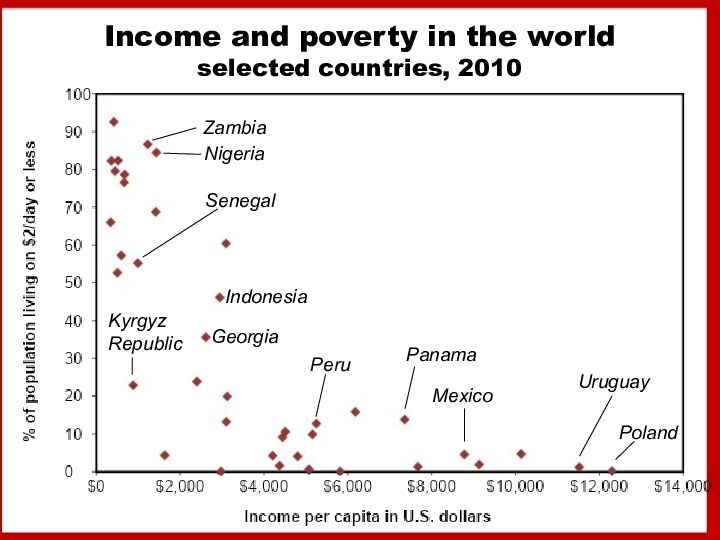
- 5. Income and poverty in the world selected countries, 2010IndonesiaUruguayPolandSenegalKyrgyz RepublicNigeriaZambiaPanamaMexicoGeorgiaPeru
- 6. 8-1 The Accumulation of CapitalThe Supply and
- 7. y = Y/L is output per worker
- 8. The Production FunctionThe PF shows how the
- 9. 8-1 The Accumulation of CapitalThe Supply and
- 10. 8-1 The Accumulation of CapitalThe Supply and
- 11. 8-1 The Accumulation of CapitalThe Supply and
- 12. 8-1 The Accumulation of CapitalThe Supply and
- 13. Output, Consumption, and InvestmentThe saving rate s
- 14. Depreciation is a constant fraction of the
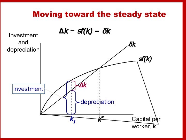
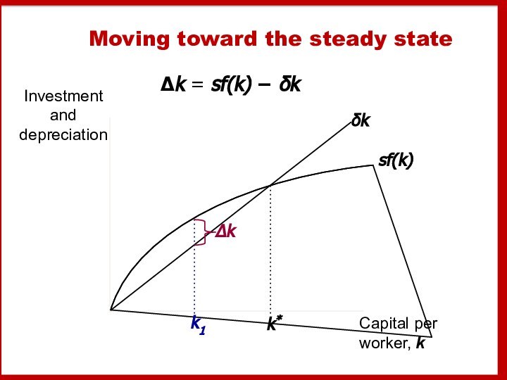
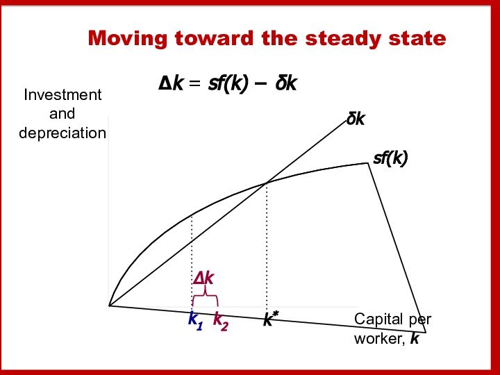
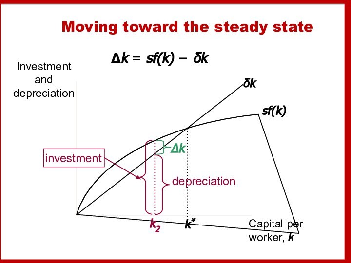
- 15. Capital accumulationChange in capital stock = investment –
- 16. The equation of motion for kThe Solow
- 17. The steady stateIf investment is just enough
- 18. The steady state
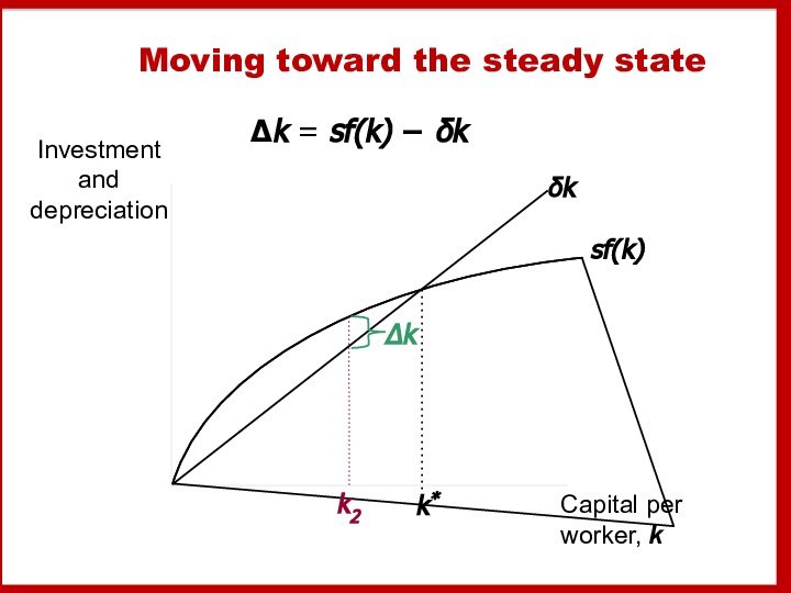
- 19. Moving toward the steady stateΔk = sf(k) − δk
- 20. Moving toward the steady stateΔk = sf(k) − δk
- 21. Moving toward the steady stateΔk = sf(k) − δkk2
- 22. Moving toward the steady stateΔk = sf(k) − δkk2
- 23. Moving toward the steady stateΔk = sf(k) − δk
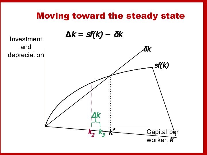
- 24. Moving toward the steady stateΔk = sf(k) − δkk2k3
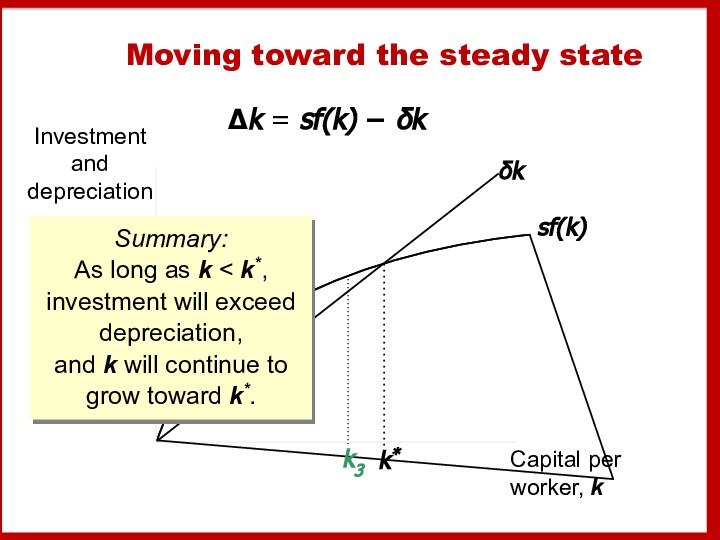
- 25. Moving toward the steady stateΔk = sf(k)
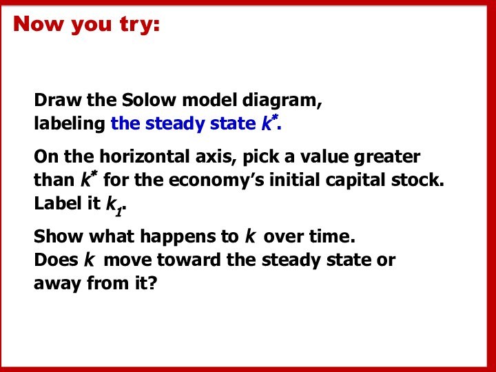
- 26. Now you try:Draw the Solow model diagram,
- 27. A numerical exampleProduction function (aggregate):To derive the
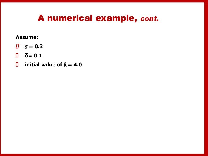
- 28. A numerical example, cont.Assume:s = 0.3δ= 0.1initial value of k = 4.0
- 29. Approaching the steady state: A numerical
- 30. Exercise: Solve for the steady stateContinue to
- 31. Solution to exercise:
- 32. An increase in the saving rateAn increase
- 33. Prediction:Higher s ⇒ higher k*. And
- 34. International evidence on investment rates and income
- 35. The Golden Rule: IntroductionDifferent values of s
- 36. The Golden Rule capital stockthe Golden Rule
- 37. Then, graph f(k*) and δk*,
- 38. The Golden Rule capital stockc* = f(k*)
- 39. The transition to the Golden Rule
- 40. Starting with too much capitalthen increasing c*
- 41. Starting with too little capitalthen increasing c*
- 42. Population growthAssume that the population (and labor
- 43. Break-even investment(δ + n)k = break-even investment,
- 44. The equation of motion for kWith population
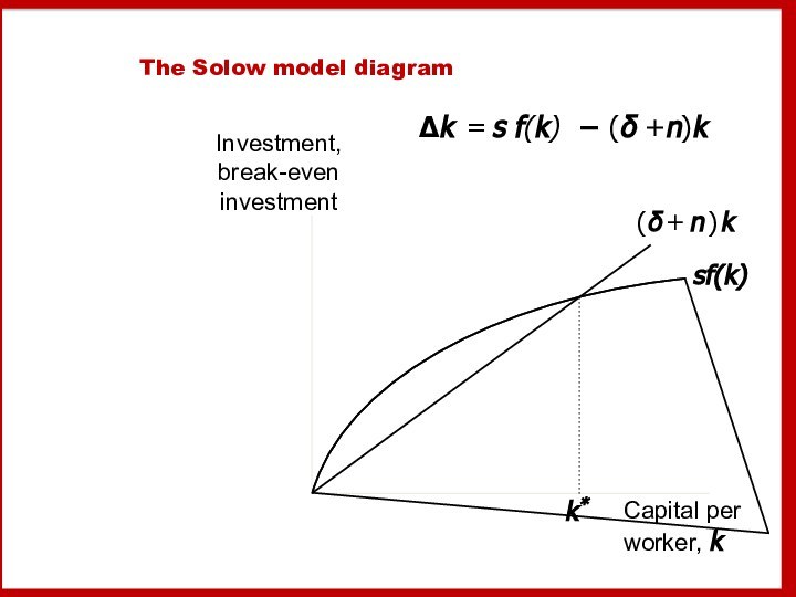
- 45. The Solow model diagramΔk = s f(k) − (δ +n)k
- 46. The impact of population growthInvestment, break-even investmentCapital
- 47. Prediction:Higher n ⇒ lower k*. And
- 48. International evidence on population growth and income
- 49. The Golden Rule with population growthTo find
- 50. Alternative perspectives on population growthThe Malthusian Model
- 51. Alternative perspectives on population growthThe Kremerian Model
- 52. Chapter Summary1. The Solow growth model shows that,
- 53. Скачать презентацию
- 54. Похожие презентации


Слайд 4
The Solow growth model shows how
saving,
population
growth,
technological progress
Level & Growth of output
A
f f e c t Слайд 5 Income and poverty in the world selected countries,
2010
Indonesia
Uruguay
Poland
Senegal
Kyrgyz Republic
Nigeria
Zambia
Panama
Mexico
Georgia
Peru
Слайд 6
8-1 The Accumulation of Capital
The Supply and Demand
for Goods
Growth in the Capital Stock and the Steady
StateApproaching the Steady State: A Numerical Example
How Saving Affects Growth
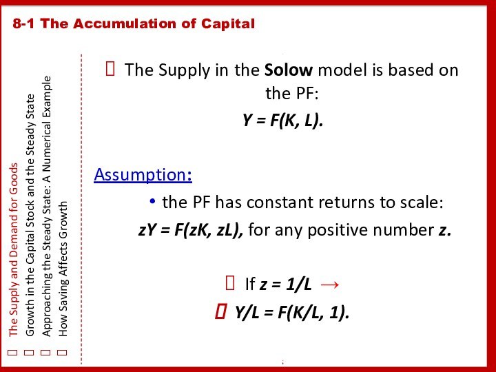
The Supply in the Solow model is based on the PF:
Y = F(K, L).
Assumption:
the PF has constant returns to scale:
zY = F(zK, zL), for any positive number z.
If z = 1/L →
Y/L = F(K/L, 1).
Слайд 7
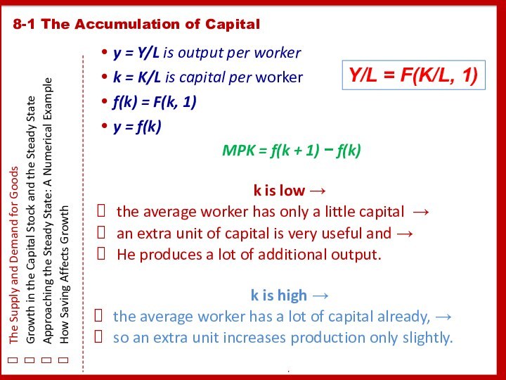
y = Y/L is output per worker
k
= K/L is capital per worker
f(k) = F(k,
1)y = f(k)
MPK = f(k + 1) − f(k)
k is low →
the average worker has only a little capital →
an extra unit of capital is very useful and →
He produces a lot of additional output.
k is high →
the average worker has a lot of capital already, →
so an extra unit increases production only slightly.
8-1 The Accumulation of Capital
The Supply and Demand for Goods
Growth in the Capital Stock and the Steady State
Approaching the Steady State: A Numerical Example
How Saving Affects Growth
Y/L = F(K/L, 1)
Слайд 8
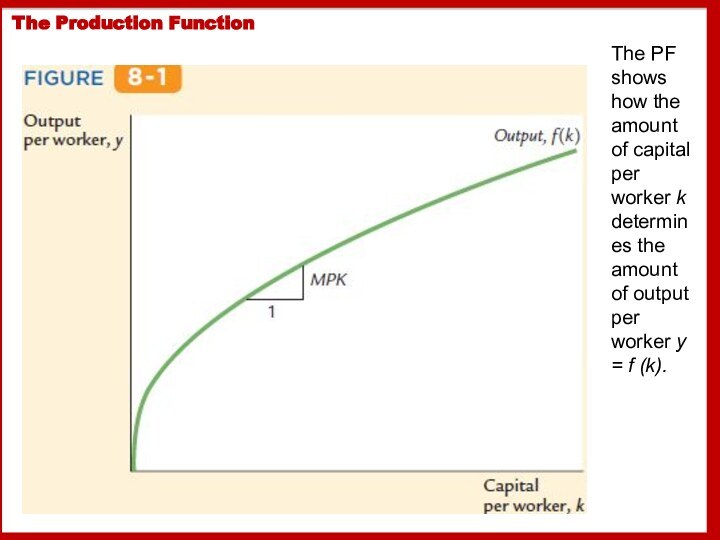
The Production Function
The PF shows how the amount
of capital per worker k determines the amount of
output per worker y = f (k).
Слайд 9
8-1 The Accumulation of Capital
The Supply and Demand
for Goods
Growth in the Capital Stock and the Steady
StateApproaching the Steady State: A Numerical Example
How Saving Affects Growth
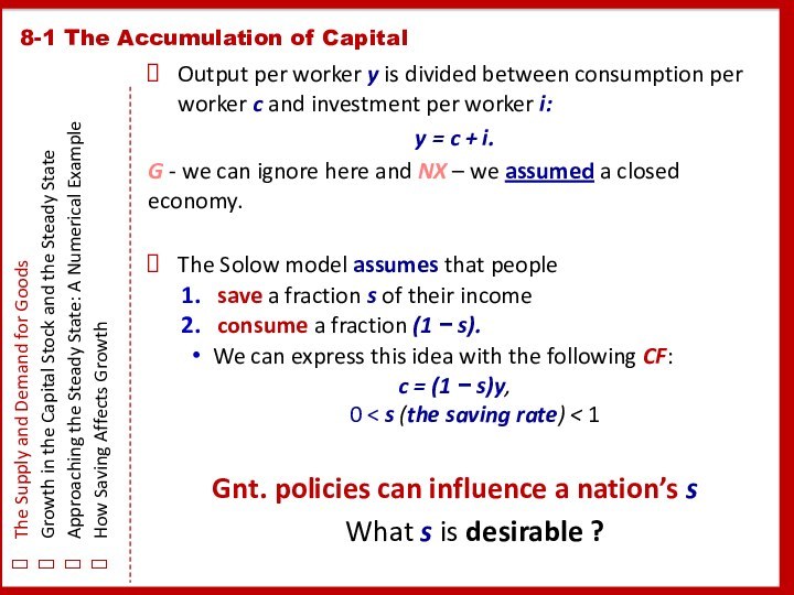
Output per worker y is divided between consumption per worker c and investment per worker i:
y = c + i.
G - we can ignore here and NX – we assumed a closed economy.
The Solow model assumes that people
save a fraction s of their income
consume a fraction (1 − s).
We can express this idea with the following CF:
c = (1 − s)y,
0 < s (the saving rate) < 1
Gnt. policies can influence a nation’s s
What s is desirable ?
Слайд 10
8-1 The Accumulation of Capital
The Supply and Demand
for Goods
Growth in the Capital Stock and the Steady
StateApproaching the Steady State: A Numerical Example
How Saving Affects Growth
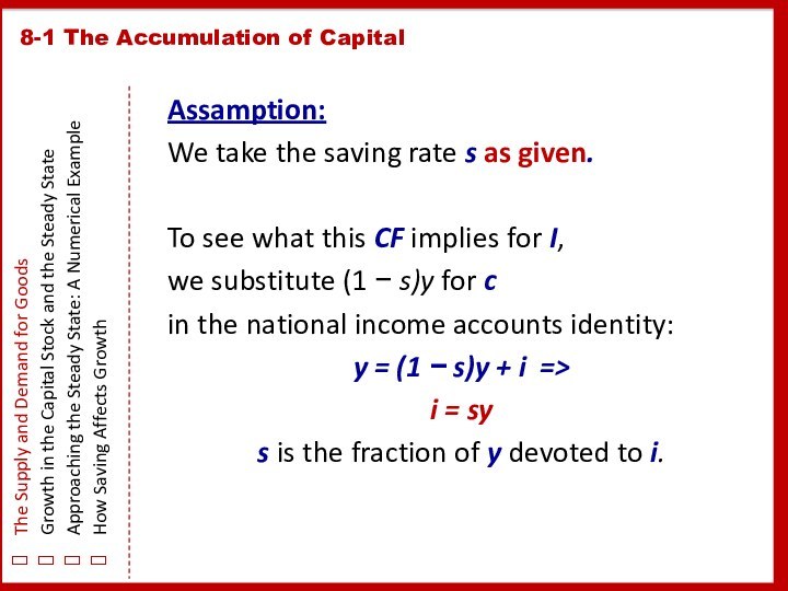
Assamption:
We take the saving rate s as given.
To see what this CF implies for I,
we substitute (1 − s)y for c
in the national income accounts identity:
y = (1 − s)y + i =>
i = sy
s is the fraction of y devoted to i.
Слайд 11
8-1 The Accumulation of Capital
The Supply and Demand
for Goods
Growth in the Capital Stock and the Steady
StateApproaching the Steady State: A Numerical Example
How Saving Affects Growth
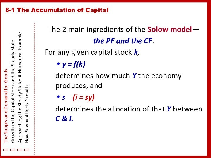
The 2 main ingredients of the Solow model—
the PF and the CF.
For any given capital stock k,
y = f(k)
determines how much Y the economy produces, and
s (i = sy)
determines the allocation of that Y between C & I.
Слайд 12
8-1 The Accumulation of Capital
The Supply and Demand
for Goods
Growth in the Capital Stock and the Steady
StateApproaching the Steady State: A Numerical Example
How Saving Affects Growth
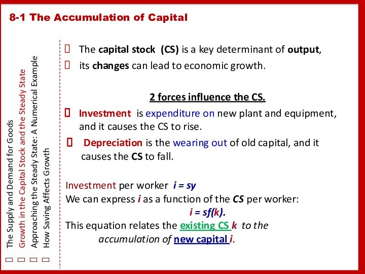
The capital stock (CS) is a key determinant of output,
its changes can lead to economic growth.
2 forces influence the CS.
Investment is expenditure on new plant and equipment, and it causes the CS to rise.
Depreciation is the wearing out of old capital, and it causes the CS to fall.
Investment per worker i = sy
We can express i as a function of the CS per worker:
i = sf(k).
This equation relates the existing CS k to the
accumulation of new capital i.
Слайд 13
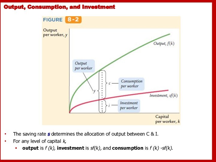
Output, Consumption, and Investment
The saving rate s determines
the allocation of output between C & I.
For
any level of capital k, output is f (k), investment is sf(k), and consumption is f (k) -sf(k).
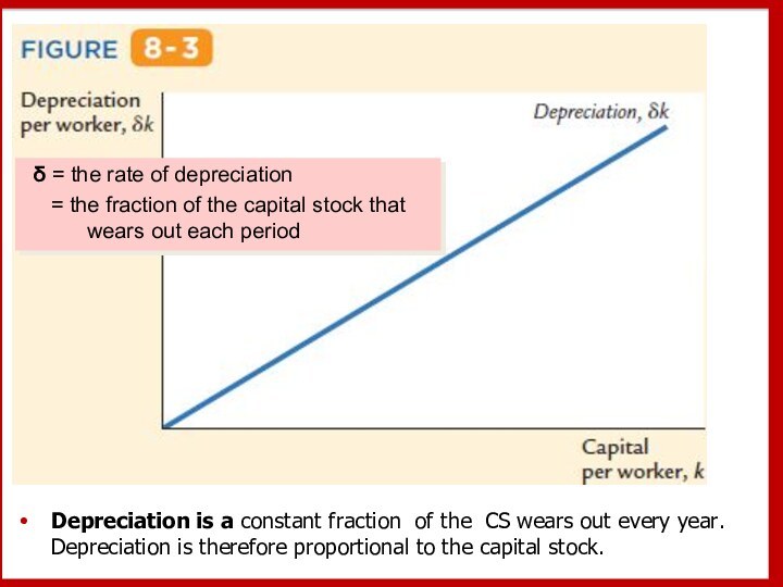
Слайд 14 Depreciation is a constant fraction of the CS
wears out every year. Depreciation is therefore proportional to
the capital stock.δ = the rate of depreciation
= the fraction of the capital stock that wears out each period
Слайд 15
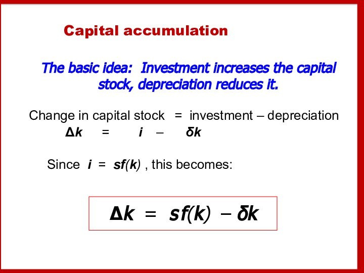
Capital accumulation
Change in capital stock = investment – depreciation
Δk
= i – δk
Since
i = sf(k) , this becomes:Δk = s f(k) – δk
The basic idea: Investment increases the capital stock, depreciation reduces it.
Слайд 16
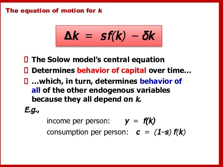
The equation of motion for k
The Solow model’s
central equation
Determines behavior of capital over time…
…which, in turn,
determines behavior of
all of the other endogenous variables
because they all depend on k. E.g.,
income per person: y = f(k)
consumption per person: c = (1–s) f(k)
Δk = s f(k) – δk
Слайд 17
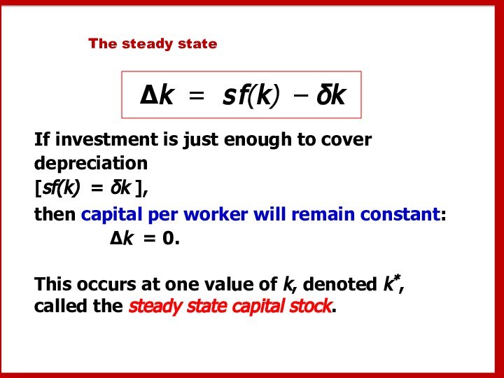
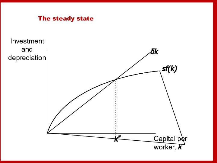
The steady state
If investment is just enough to
cover depreciation
[sf(k) = δk ],
then capital per
worker will remain constant:
Δk = 0. This occurs at one value of k, denoted k*, called the steady state capital stock.
Δk = s f(k) – δk
Слайд 25
Moving toward the steady state
Δk = sf(k) −
δk
k3
Summary:
As long as k < k*, investment will exceed
depreciation,
and k will continue to grow toward k*.
Слайд 26
Now you try:
Draw the Solow model diagram,
labeling
the steady state k*.
On the horizontal axis, pick
a value greater than k* for the economy’s initial capital stock. Label it k1. Show what happens to k over time. Does k move toward the steady state or away from it?
Слайд 27
A numerical example
Production function (aggregate):
To derive the per-worker
production function, divide through by L:
Then substitute y =
Y/L and k = K/L to get
Слайд 29
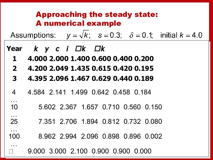
Approaching the steady state:
A numerical example
Year
k y c i k
k1 4.000 2.000 1.400 0.600 0.400 0.200
2 4.200 2.049 1.435 0.615 0.420 0.195
3 4.395 2.096 1.467 0.629 0.440 0.189
4 4.584 2.141 1.499 0.642 0.458 0.184
…
10 5.602 2.367 1.657 0.710 0.560 0.150
…
25 7.351 2.706 1.894 0.812 0.732 0.080
…
100 8.962 2.994 2.096 0.898 0.896 0.002
…
9.000 3.000 2.100 0.900 0.900 0.000
Слайд 30
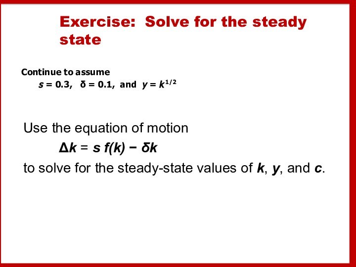
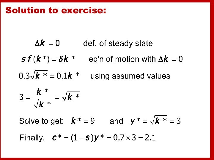
Exercise: Solve for the steady state
Continue to assume
s = 0.3, δ = 0.1, and y
= k 1/2Use the equation of motion
Δk = s f(k) − δk
to solve for the steady-state values of k, y, and c.
Слайд 32
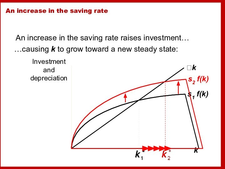
An increase in the saving rate
An increase in
the saving rate raises investment…
…causing k to grow toward
a new steady state:
Слайд 33
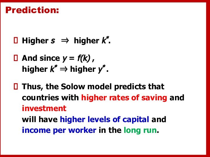
Prediction:
Higher s ⇒ higher k*.
And since
y = f(k) , higher k* ⇒ higher y*
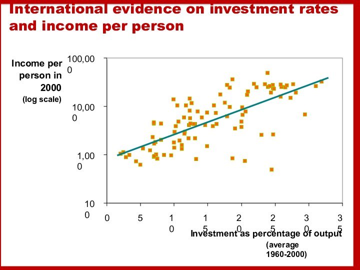
.Thus, the Solow model predicts that countries with higher rates of saving and investment will have higher levels of capital and income per worker in the long run.
Слайд 34 International evidence on investment rates and income per
person
100
1,000
10,000
100,000
0
5
10
15
20
25
30
35
Investment as percentage of output
(average 1960-2000)
Income per
person
in 2000
(log scale)
Слайд 35
The Golden Rule: Introduction
Different values of s lead
to different steady states. How do we know which
is the “best” steady state?The “best” steady state has the highest possible consumption per person: c* = (1–s) f(k*).
An increase in s
leads to higher k* and y*, which raises c*
reduces consumption’s share of income (1–s), which lowers c*.
So, how do we find the s and k* that maximize c*?
Слайд 36
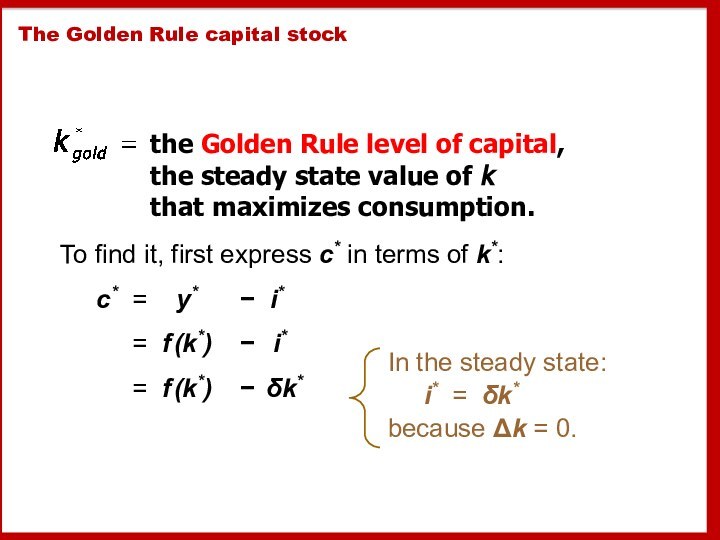
The Golden Rule capital stock
the Golden Rule level
of capital, the steady state value of k that
maximizes consumption.To find it, first express c* in terms of k*:
c* = y* − i*
= f (k*) − i*
= f (k*) − δk*
In the steady state: i* = δk* because Δk = 0.
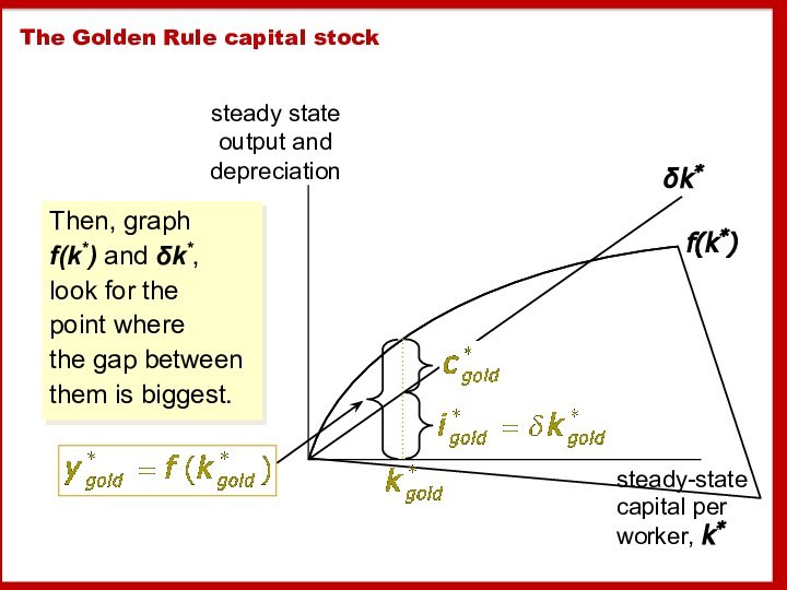
Слайд 37 Then, graph f(k*) and δk*, look for the
point where
the gap between them is biggest.
The
Golden Rule capital stock
Слайд 38
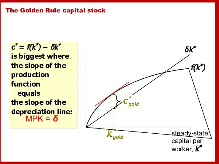
The Golden Rule capital stock
c* = f(k*) −
δk* is biggest where the slope of the production function
equals the slope of the depreciation line:steady-state capital per
worker, k*
MPK = δ
Слайд 39
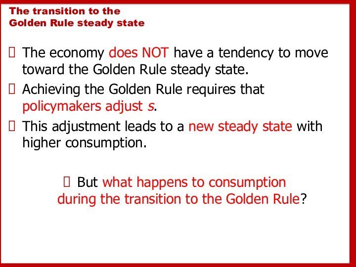
The transition to the
Golden Rule steady state
The
economy does NOT have a tendency to move toward
the Golden Rule steady state.Achieving the Golden Rule requires that policymakers adjust s.
This adjustment leads to a new steady state with higher consumption.
But what happens to consumption during the transition to the Golden Rule?
Слайд 40
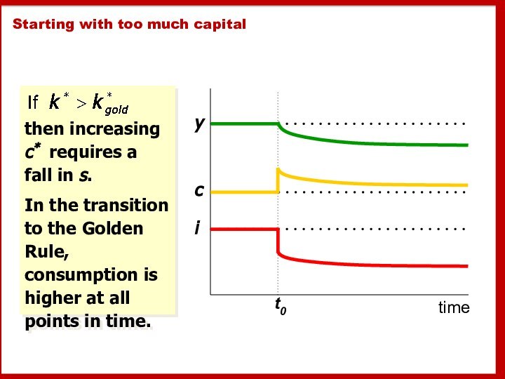
Starting with too much capital
then increasing c* requires
a fall in s.
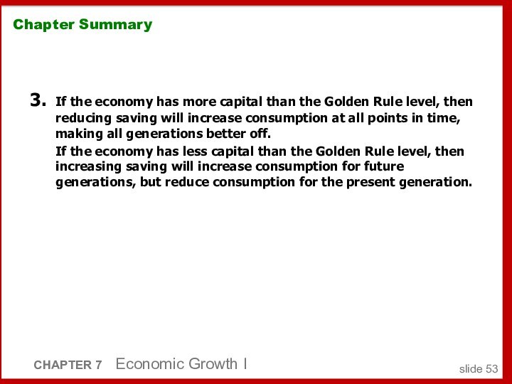
In the transition to the
Golden Rule, consumption is higher at all points in time.t0
c
i
y
Слайд 41
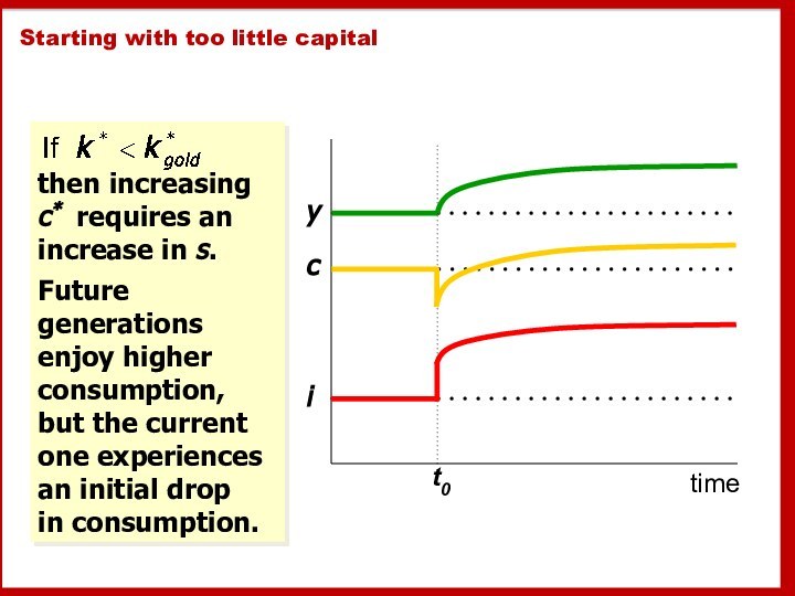
Starting with too little capital
then increasing c* requires
an
increase in s.
Future generations
enjoy higher consumption,
but the current
one experiences
an initial drop
in consumption.time
t0
c
i
y
Слайд 42
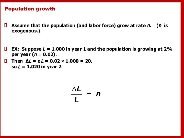
Population growth
Assume that the population (and labor force)
grow at rate n. (n is exogenous.)
EX: Suppose
L = 1,000 in year 1 and the population is growing at 2% per year (n = 0.02). Then ΔL = n L = 0.02 × 1,000 = 20, so L = 1,020 in year 2.
Слайд 43
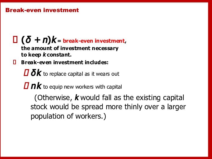
Break-even investment
(δ + n)k = break-even investment,
the
amount of investment necessary
to keep k constant.
Break-even
investment includes:δ k to replace capital as it wears out
n k to equip new workers with capital
(Otherwise, k would fall as the existing capital stock would be spread more thinly over a larger population of workers.)
Слайд 44
The equation of motion for k
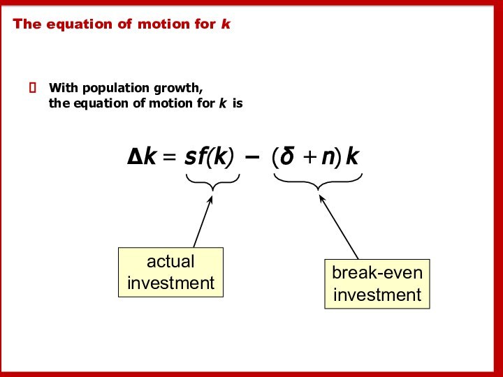
With population growth,
the equation of motion for k is
Δk = s
f(k) − (δ + n) k
Слайд 46
The impact of population growth
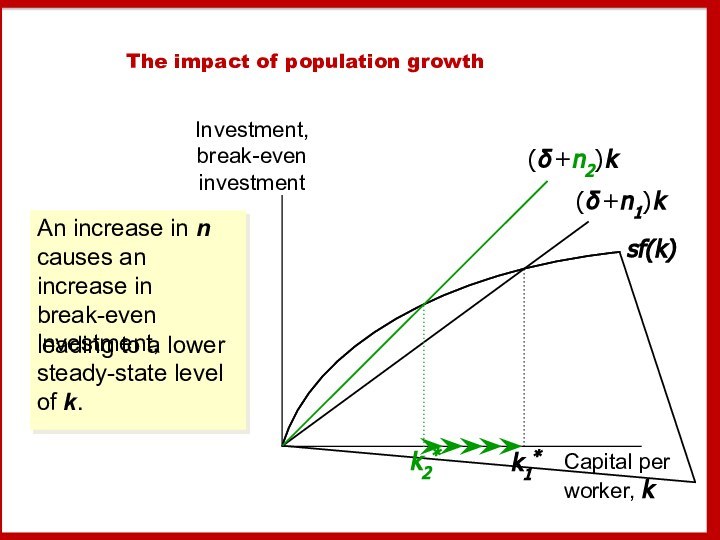
Investment, break-even investment
Capital per
worker, k
(δ +n1) k
k1*
An increase in n
causes an increase in break-even investment,leading to a lower steady-state level of k.
Слайд 47
Prediction:
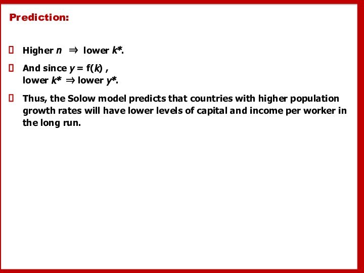
Higher n ⇒ lower k*.
And since
y = f(k) , lower k* ⇒ lower y*.
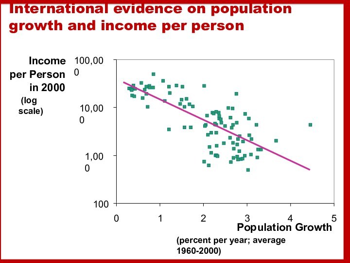
Thus, the Solow model predicts that countries with higher population growth rates will have lower levels of capital and income per worker in the long run.
Слайд 48 International evidence on population growth and income per
person
100
1,000
10,000
100,000
0
1
2
3
4
5
Population Growth
(percent per year; average 1960-2000)
Income
per Person
in 2000
(log scale)
Слайд 49
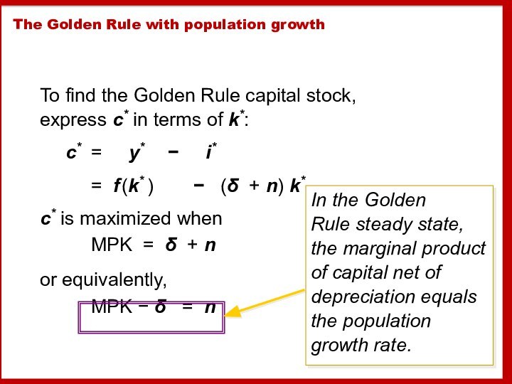
The Golden Rule with population growth
To find the
Golden Rule capital stock, express c* in terms of
k*:c* = y* − i*
= f (k* ) − (δ + n) k*
c* is maximized when MPK = δ + n
or equivalently, MPK − δ = n
In the Golden
Rule steady state,
the marginal product
of capital net of depreciation equals the population
growth rate.
Слайд 50
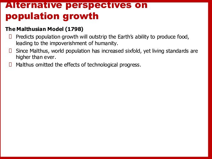
Alternative perspectives on population growth
The Malthusian Model (1798)
Predicts
population growth will outstrip the Earth’s ability to produce
food, leading to the impoverishment of humanity.Since Malthus, world population has increased sixfold, yet living standards are higher than ever.
Malthus omitted the effects of technological progress.
Слайд 51
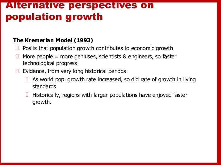
Alternative perspectives on population growth
The Kremerian Model (1993)
Posits
that population growth contributes to economic growth.
More people
= more geniuses, scientists & engineers, so faster technological progress.Evidence, from very long historical periods:
As world pop. growth rate increased, so did rate of growth in living standards
Historically, regions with larger populations have enjoyed faster growth.
Слайд 52
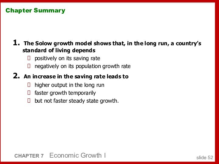
Chapter Summary
1. The Solow growth model shows that, in
the long run, a country’s standard of living depends
positively
on its saving ratenegatively on its population growth rate
2. An increase in the saving rate leads to
higher output in the long run
faster growth temporarily
but not faster steady state growth.
CHAPTER 7 Economic Growth I
slide


